📌
##########################################
# 이항 분류 : 분류의 종류가 2종류인 경우
import pandas as pd
url = "<http://archive.ics.uci.edu/ml/machine-learning-databases/wine-quality/>"
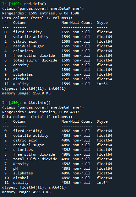
red = pd.read_csv(url + 'winequality-red.csv', sep=';') # red와인 정보
white = pd.read_csv(url + 'winequality-white.csv', sep=';') #white와인 정보
red.info()
white.info()
'''
1 - fixed acidity : 주석산농도
2 - volatile acidity : 아세트산농도
3 - citric acid : 구연산농도
4 - residual sugar : 잔류당분농도
5 - chlorides : 염화나트륨농도
6 - free sulfur dioxide : 유리 아황산 농도
7 - total sulfur dioxide : 총 아황산 농도
8 - density : 밀도
9 - pH : ph
10 - sulphates : 황산칼륨 농도
11 - alcohol : 알코올 도수
12 - quality (score between 0 and 10) : 와인등급
'''
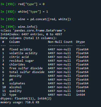
# type컬럼 추가
# red와인인 경우 type컬럼에 0, white와인인 경우 type컬럼에 1을 저장하기
red["type"] = 0
white["type"] = 1
# red, white 데이터를 합하여 wine 데이터에 저장하기
wine = pd.concat([red, white])
wine.info()
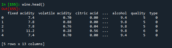
wine.head()
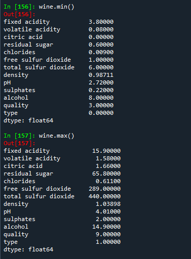
# wine 데이터를 minmax 정규화 하여 wine_norm 데이터에 저장
wine.min() # 모든 컬럼의 각각의 최소값이 나타남
wine.max() # 각 컬럼별 최대값이 나타남
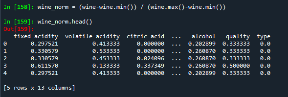
wine_norm = (wine-wine.min()) / (wine.max()-wine.min())
wine_norm.head()
wine_norm.min()
wine_norm.max()

# wine_norm 데이터를 섞어 wine_shuffle 데이터에 저장하기
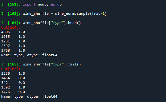
import numpy as np
wine_shuffle = wine_norm.sample(frac=1)
wine_shuffle["type"].head()
wine_shuffle["type"].tail()
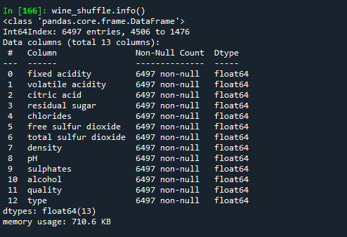
wine_shuffle.info()
# wine_shuffle 데이터를 배열데이터 wine_np로 저장
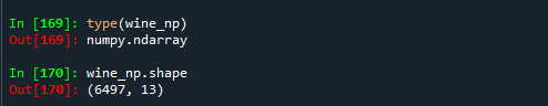
wine_np = wine_shuffle.to_numpy()
type(wine_np)
wine_np.shape
# train(8), test(0) 데이터 분리
# 설명변수, 목표변수(정답)로 분리
train_idx = int(len(wine_np)*0.8)
train_idx # 5197
train_x, train_y = \\
    wine_np[:train_idx,:-1], wine_np[:train_idx, -1]
train_x.shape
train_y.shape

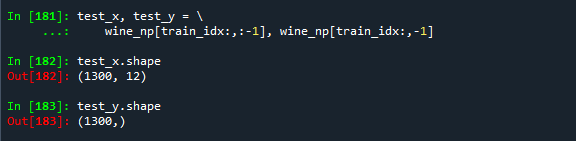
# 테스트 데이터 분리
test_x, test_y = \\
    wine_np[train_idx:,:-1], wine_np[train_idx:,-1]
test_x.shape
test_y.shape
# label을 one-hot 인코딩하기
import tensorflow as tf
train_y = tf.keras.utils.to_categorical(train_y, num_classes=2)
test_y = tf.keras.utils.to_categorical(test_y, num_classes=2)

# 모델 생성
from tensorflow.keras import Sequntial
from tensorflow.keras.layers import Dense

model = Sequential([
    Dense(units=48, activation='relu', input_shape=(12,)),
    Dense(units=24, activation='relu'),
    Dense(units=12, activation='relu'),
    Dense(units=2, activation='sigmoid') # 이중분류 사용.
    ])
model.summary()
# binary_crossentropy : 이중분류에서 사용되는 손실함수
#                       레이블을 one-hot 인코딩 필요.
model.compile(optimizer="adam", loss='binary_crossentropy', metrics=['accuracy'])
# validation_split=0.25 : 25%의 데이터를 검증데이터로 사용
history = model.fit(train_x, train_y, epochs=25, batch_size=32,\\
                    validation_split=0.25
# 학습결과 시각화 하기
# 학습데이터와 검증데이터의 loss, accuracy 값을 선그래프로 출력하기
import matplotlib.pyplot as plt
plt.figure(figsize=(12,4))
plt.subplot(1, 2, 1)
plt.plot(history.history['loss'], 'b-', label='loss')
plt.plot(history.history['val_loss'],'r--', label='accuracy')
plt.xlabel('Epoch')
plt.legend()

plt.subplot(1,2,2)
plt.plot(history.history['accuracy'],'b-', label='accuracy')
plt.plot(history.history['val_accuracy'],'r--', label='val_accuracy')
plt.xlabel('Epoch')
plt.ylim(0.7,1)
plt.legend()
plt.show()
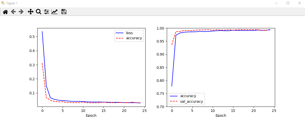
# 과적합 발생 안됨.
# 평가하기
model.evaluate(test_x, test_y) # [0.02699071355164051, 0.9938461780548096]
# 예측하기
results = model.predict(test_x)
# 평가 결과 출력하기 : 혼동행렬, heatmap 출력하기
# 혼동행렬(confusion_matrix)
from sklearn.metrics import confusion_matrix
cm = confusion_matrix(np.argmax(test_y, axis=-1), \\
np.argmax(results, axis=-1))
cm
import seaborn as sns
plt.figure(figsize=(7, 7))
sns.heatmap(cm, annot = True, fmt = 'd', cmap = 'Blues')
plt.xlabel('predicted label', fontsize=15)
plt.ylabel('true label', fontsize=15)
plt.xticks(range(2), ['red', 'white'], rotation=45)
plt.yticks(range(2), ['red', 'white'], rotation=0)
plt.show()
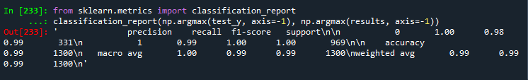
from sklearn.metrics import classification_report
classification_report(np.argmax(test_y, axis=-1), np.argmax(results, axis=-1))

'수업(국비지원) > Python' 카테고리의 다른 글
| [Python] 컬러 이미지 분석하기 (0) | 2023.04.27 |
|---|---|
| [Python] 2023-01-02 복습 (0) | 2023.04.27 |
| [Python] Fashion-MNIST 데이터를 이용하여 예측 평가하기 (0) | 2023.04.27 |
| [Python] MNIST 데이터를 이용하여 숫자를 학습하여 숫자 인식 (0) | 2023.04.27 |
| [Python] Tensortflow (0) | 2023.04.27 |


